本文共 6854 字,大约阅读时间需要 22 分钟。
做了好几天的面试题,发现 String 类的题目一直是个大头,看似简单,实则不然,牵扯到很多底层的东西。接下来我就跟着源码和题目来分析一下把
一、String的对象不可变
public final class String implements java.io.Serializable, Comparable, CharSequence { /** The value is used for character storage. */ private final char value[];
可以看到,String 类是被 final 修饰的,即 String 类不能被继承。其中有一个很重要的数组,char 数组,用来保存字符串的,既然是用 final 关键字来修饰的,那就代表 String 是不可变的
举以下两个方法为例,通过源代码可以看到,substring,replace 最后都是通过 new String(xxx) 来产生了一个新的 String 对象,最原始的字符串并没有改变
public String substring(int beginIndex, int endIndex) { if (beginIndex < 0) { throw new StringIndexOutOfBoundsException(beginIndex); } if (endIndex > value.length) { throw new StringIndexOutOfBoundsException(endIndex); } int subLen = endIndex - beginIndex; if (subLen < 0) { throw new StringIndexOutOfBoundsException(subLen); } return ((beginIndex == 0) && (endIndex == value.length)) ? this : new String(value, beginIndex, subLen);}public String replace(char oldChar, char newChar) { if (oldChar != newChar) { int len = value.length; int i = -1; char[] val = value; /* avoid getfield opcode */ while (++i < len) { if (val[i] == oldChar) { break; } } if (i < len) { char buf[] = new char[len]; for (int j = 0; j < i; j++) { buf[j] = val[j]; } while (i < len) { char c = val[i]; buf[i] = (c == oldChar) ? newChar : c; i++; } return new String(buf, true); } } return this;} 我们可以用例子验证一下:
public void stringTest3(){ String a = "nihaoshije"; String b = a.substring(0, 4); System.out.println(b); System.out.println(a);} 最终的输出为:niha nihaoshije。可见如我们所预料的,原来的 String 的值并没有改变
二、StringBuilder 中的字符可变
我们可以通过 StringBuilder 的源码分析下
我们假设使用 append 方法,该方法返回的依然是 StringBuffer 对象本身,说明他确实是值改变了
public StringBuilder append(String str) { super.append(str); return this;} 该方法实际调用的是 StringBuilder 的父方法。该父方法,会先检测容量够不够,不够的话会进行扩容,然后调用 String 的 getChars 方法。注意,最后返回的依旧是 StringBuffer 对象
public AbstractStringBuilder append(String str) { if (str == null) return appendNull(); int len = str.length(); ensureCapacityInternal(count + len); str.getChars(0, len, value, count); count += len; return this;} getChars 方法具有 4 个参数
- srcBegin – 字符串中要复制的第一个字符的索引。
- srcEnd – 字符串中要复制的最后一个字符之后的索引。
- dst – 目标数组。
- dstBegin – 目标数组中的起始偏移量。
其中的 dst 对应 StringBuilder 的父类里的数组 char[] value,该数组是专门用来存放字符的。append(String str) 里的字符串就是以字符格式一个个加到 char 数组里的
public void getChars(int srcBegin, int srcEnd, char dst[], int dstBegin) { if (srcBegin < 0) { throw new StringIndexOutOfBoundsException(srcBegin); } if (srcEnd > value.length) { throw new StringIndexOutOfBoundsException(srcEnd); } if (srcBegin > srcEnd) { throw new StringIndexOutOfBoundsException(srcEnd - srcBegin); } System.arraycopy(value, srcBegin, dst, dstBegin, srcEnd - srcBegin);} 我们可以举一个例子来看一下 StringBuffer 的对象是否真正改变了
public void stringBuilderTest() { StringBuilder stringBuilder = new StringBuilder("hello"); System.out.println(stringBuilder); stringBuilder.append("world"); System.out.println(stringBuilder);} 第一输出为 hello,第二次再次输出同一个对象,变为 helloworld,结果一目了然
三、关于字符串相加
这里我讨论的是使用“+”对两个字符串相加的过程,看似很简单的相加,其实蕴藏着很多的密码
《Java编程思想》提到,String 对象的操作符“+”其实被赋予了特殊的含义,该操作符是 Java 中仅有的两个重载过的操作符。而通过反编译可以看到,String 对象在进行“+”操作的时候,其实是调用了 StringBuilder 对象的 append() 方法来加以构造
按照惯例,我们先来看两个字符串相加的例子
public void stringTest4(){ String a1 = "helloworld"; String a = "hello" + "world"; String b = "hello"; String c = "world"; String d = b + c; System.out.println(a); System.out.println(d); System.out.println(a == d); System.out.println(a1 == a); System.out.println(a1 == d);} 输出结果如下
helloworldhelloworldfalsetruefalse
先来看 String a,“hello” + “world” 在 String 编译期间进行优化,优化结果为 “helloworld”,而该值在常量池中已经存有一份,因此 a 也指向了该常量池中的字符串,因此 a1 和 a 相等,输出 true
在对 b 和 c 进行相加的过程中,其实是分两个步骤来进行。先是调用 StringBuilder 对象的 append() 方法,加上 “hello” 字符;然后在调用一次 append() 方法,加上 “world”,最后默认调用 StringBuilder 的 toString() 方法输出“helloworld”。
很明显 d 对象指向的是堆中的 String 对象,而 a1 则指向的是常量池中的字符串,两者引用明显不同,因此输出 false。a 和 d 的比较与之类似,这里不加以赘述
我用反编译来看一下直接字符串相加和使用引用相加的区别
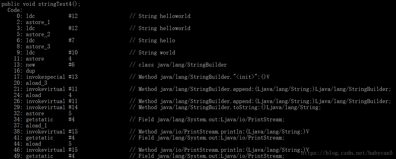 这里我就抽取了一部分反编译的结果。
 1).可以看到,在第0行的时候,字符串就已经变成 helloworld 了,说明 “hello” + “world” 在编译的期间就已经进行了优化
2). 第13行开始,也就是在执行 b+c 这个语句的时候,就开始调用 append() 的方法了。当执行到 b 的时候,创建一个 StringBuilder 对象,调用 append() 方法加入,当执行到 c 的时候,再次调用 append() 加入。此时完成相加,以 String 类型返回。b + c 返回的结果相当于存入了一个新的 String 对象,最后在用变量 d 指向这个新的对象
3). 关于相加的效率,那么字符串引用相加(a + b)的效率,会比直接相加低,因为编译器不会对引用变量加以优化
四、String、StringBuffer、StringBuilder 对比
执行效率
StringBuilder > StringBuffer > String
当然这个是相对的,不一定在所有情况下都是这样。
比如String str = “hello” + "world"的效率就比 StringBuilder st = new StringBuilder().append(“hello”).append(“world”)要高。
因此,如果是字符串相加操作或者改动较少的情况下,使用 String str = "hello" + "world" + ... 这种形式;土改时字符串相加比较多的话,建议使用 StringBuilder
线程安全
StringBuffer 线程安全的,StringBuilder 不是线程安全的
@Overridepublic synchronized StringBuffer append(Object obj) { toStringCache = null; super.append(String.valueOf(obj)); return this;} public StringBuilder append(StringBuffer sb) { super.append(sb); return this;} 五、常见的面试题目
1.输出以下结果
String a = "hello";String b = "hello";String a1 = new String("hello");String a2 = new String("hello");StringBuilder c = new StringBuilder("hello");StringBuilder d = new StringBuilder("hello");a == ba1 == a2c == da1.equals(a2)a1.equals(c)a.equals(c)c.equals(d) 答案为 true、false、false、true、false、false。
a 和 b 指向同一个常量池,由此相等;a1 和 a2,c 和 d 都是因为对象不同所以不等;a1 和 a2 同属于 String 类型且字符相等;a1 和 c ,a 和 c 因为类型不同所以直接返回 false; c 和 d 因为对象不同返回 false。2.输出以下结果
String a = "hellonihao";String b = "hello" + "nihao";a == b
输出结果为 true。原因上面也提到了,“hello” + “nihao” 在编译的过程中就已经优化成了 “hellonihao”,此时常量池中已经有一个 “hellonihao”,这个时候不要再去新建一个对象,因此 a 和 b 指向的是同一个对象
3.输出以下结果
String a = "nihaoshijie";String b = "nihao";String c = "shijie";String d = b + c;a == d
输出结果为 false。因为"+"在Java中是重载运算符,String 对象直接相加的过程不会在编译期间优化,相加的结果会保存在一个新的对象中,因此 a 和 d 指向的根本不是一个对象
4.输出以下结果
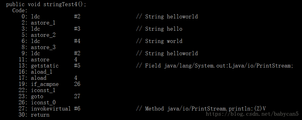
String a = "helloworld";final String b = "hello";final String c = "world";String d = b + c;a == d;
输出结果居然是 true。对于被 final 修饰符修饰的变量,一经修饰便不能改变此时这两个 String 对象 b 和 c 在相加的过程中都能指向其他对象了。因此 String d = b + c 在编译期间就会被优化成:String d = "hello" + "world" = "helloworld",而这个常量在常量池已经有了,因此返回 true。下面是反编译的验证
5.输出以下结果
String a = "hello";String b = new String("hello");String c = a.intern();a == b;a == c; 结果为false、true。第一个很好理解;第二个的话,由于常量池中已经存在了 “hello” 这个字符串,所以直接返回该字符串的引用
intern():
当调用 intern 方法时,如果池已经包含一个等于此 String 对象的字符串(该对象由 equals(Object) 方法确定),则返回池中的字符串。否则,将此 String 对象添加到池中,并且返回此 String 对象的引用。它遵循对于任何两个字符串 s 和 t,当且仅当 s.equals(t) 为 true 时,s.intern() == t.intern() 才为 true。
对一个字符串调用intern()方法后,会先检查池内是否有该字符串,若有则返回;若没有没有则先创建再返回,确保返回的字符串已经以字面量的形式存在于池中。